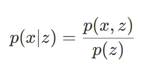
Scary Formula

Most of the time, while reading papers, I’ve struggled to fully understand this expression:

Every time I think, "Okay! Now I’ve finally grasped this formula," I find myself going back to it again later.
So, I’m writing the version that I understood today — in plain language. I’ll build up to generative models progressively, starting with the basics. Let’s get to it.

Level 1: Intuition Building

The expression simply reads as “probability of x given z”.
We are given z, and we want to find how likely x is under that condition.
In other words: in a world where z is known to be true, how likely is it that xalso happens?

Real-Life Example

Suppose:

• z = "graduated"
• x = "got a job"

Then the expression p(x|z) asks:

Given that a student graduated, what are the chances they get a job?

Assume there are only two outcomes for a graduate:

• They get a job
• Or they don’t

We're interested in:

This is a conditional probability — meaning we are calculating probability given that something has already happened.

Out of all the students who graduated, how likely is it that one gets a job?

Now imagine we live in a world where everyone has already graduated.
In that world, we want to ask:

Who among them actually got a job?

For everyone who did, one thing is certain:

They both graduated and got a job.

So, this is:

It’s just counting the people who satisfy both events simultaneously.

Different Combinations

Since both x and z are binary (job/no job, graduated/not), we have four possibilities:

• Got a job, given graduated
• Didn't get a job, given graduated
• Got a job, given not graduated
• Didn't get a job, given not graduated

Even though reality has many combinations, this formula lets us zoom into the specific world we care about — here, the group of graduates.

So we’re focused on:

Now your intuition might say:

"Wait — this is just a fraction!"

You're right.

We’re asking:

Out of (X), how many were (Y)?

This is simply:

Where:

• X = p(z = "graduated") — the total number of graduates
• Y = p(x = "got job", z = "graduated") — the number who got a job and graduated

So:

Other Cases

Similarly:

General Case

We write this as:

Which assumes:

We are narrowing down the world to a subset (like graduates), and asking what happens within that subset.

Flipping It: What About p(z | x)?

Let’s now reverse the perspective.

Out of the people who got a job, how many had graduated?

That’s asking for:

Which is:

So we now have both:

This symmetry is what makes Bayes’ Rule feel magical.
We simply walked in through the other door of the same house.

Level 2: Distribution Thinking

The one utmost important thing about probability is that it brings the idea of distribution with it.
So whenever we see p(x), read as the probability of an event (x), we should remember that this value is tied to a distribution.

Due to my weak fundamentals, I used to think that p(x) was just a number, something we measure or calculate through some real-world experiments.
While that's partially true, everything started making sense to me once I started thinking about probability in terms of how things are distributed, not just measured.

The following part is so interesting 😄!

Not Just a Number — a Shape

In Level 1, we treated the conditional probability like a simple fraction.
Something like: Out of all students who graduated, how many of them got a job?

For intuition building, this works well.
But now let's pause here and ask a deeper question:

Where do these numbers (values of each probability) come from?

For example:

But what is this 0.4, really?
Is it just a number someone gives us? Or is it part of something bigger?

Turns out, it's a part of a distribution — a full picture of how people are spread across different possible outcomes.

To make it clear, let's revisit our previous example.
We have only two variables:

• $x$: whether someone got a job (yes or no)
• $z$: whether someone graduated (yes or no)

Since both of these are binary, the total number of possible combinations is just four.
And each of those combinations happens with a certain likelihood — some are common, some are rare.

Each one has its probability value — and together, they form a joint distribution $p(x, z)$.

Visualizing the Discrete Distribution

To help you see this, here's a 3D plot of our joint distribution:

Each block represents one of the four possible outcomes, and the height of the block shows how likely that scenario is in our population.

You can think of it like a tiny 3D city:

• Taller blocks = more people fall into that category
• Shorter blocks = fewer people
• And if you add up the height of all four blocks, you get 1 — because everyone has to land somewhere

So when we write something like p(x, z), we're no longer talking just about a number.
We are talking about one specific point in this 3D landscape. The height represents how much of the real world lives there.

This was the mental shift that changed everything for me:

A probability is not just a measurement — it's a shape. It shows how reality is distributed.

So from the above plot, we can derive these values:

$p(x=1, z=0) = 0.3$
$p(x=1, z=1) = 0.4$
$p(x=0, z=0) = 0.2$
$p(x=0, z=1) = 0.1$

$p(x=0) = p(x=0,z=0) + p(x=0,z=1) = 0.2 + 0.1 = 0.3$
$p(x=1) = 0.7$
$p(z=0) = 0.5$
$p(z=1) = 0.5$
$p(x=1 | z=1) = p(x=1, z=1) / p(z=1) = 0.4 / 0.5 = 0.8$

The visualization of the example we took was easy because:

• The variables $x$ and $z$ were binary, which intrinsically means they are discrete
• The discrete cases are easy to visualize as we just have to pick the correct box from the probability distribution — it's like selecting from a fixed menu

Continuous World

But if we now make this same example a continuous one, then we need to make a few tweaks in how we think about things — both mathematically and visually.

Instead of just asking whether someone got a job or not, let's ask:

How long did it take them to get a job after graduation?

Now, instead of $x$ being just 0 or 1, it could be any number — like 2.5 months, 4.8 months, or 7.1 months.
That makes $x$ a continuous variable.

Here's the twist:
In the discrete world, we could assign a clean value like:

But in the continuous world, the probability of any single, exact value (like $x = 4.8$) is basically zero.

Why? Because there are infinitely many possible values that $x$ can take.
Out of these infinite possibilities, the chance that it lands on one specific value is so small that it's considered zero.

Let me make that clearer:

In the continuous world, we don't ask questions like:

• What's the probability that a person gets a job exactly on July 2nd?
• What's the probability that John eats rice at exactly 4:54 PM?

These are exact points in time.
While something might happen at those times in real life, the theoretical probability assigned to that single point is zero.
Not because it's impossible — but because it's infinitely narrow, like picking one grain of sand from an endless beach.

So in continuous probability, we always think in ranges, not points. We ask:

• What's the probability that someone got a job between month 4 and month 6?
• Or that John eats rice between 4:50 PM and 5:00 PM?

So instead of thinking in terms of fixed values, we now think in terms of ranges.

Visualizing the Continuous Distribution

Visualizing a continuous distribution isn't so different from visualizing a discrete one.
The key difference is:

Instead of a few separate bars, we now imagine an infinite number of bars packed so closely together that they form a smooth surface.

Think of it like this:

Take the 3D bar plot we used earlier (the one with four separate blocks), and imagine placing a blanket over it.
Now, imagine the bars becoming thinner and thinner — and more and more of them appearing — until the blanket settles perfectly on top with no gaps.

The result is a smooth, continuous surface.

That's what a continuous distribution looks like — smooth and gapless — because the variables can take any value within a range, not just a few fixed ones like in the binary case.

To put it simply, the main differences between discrete (binary) and continuous distributions are:

• In the binary case, variables can take only one of two values (like 0 or 1)
• In the continuous case, variables can take any value within a given range (like 2.5, 4.81, 6.013, etc.)
• In discrete plots, we visualize individual bars, while in continuous ones, we imagine a smooth curve or surface

And just like in the discrete case, where the height of each bar tells us how likely that scenario is,
in the continuous case, the height of the curve at any point tells us how dense the probability is around that value.

The total area under the curve still adds up to 1 — just like the total height of all bars did in the discrete case.

Conditional Probability for Continuous Variables

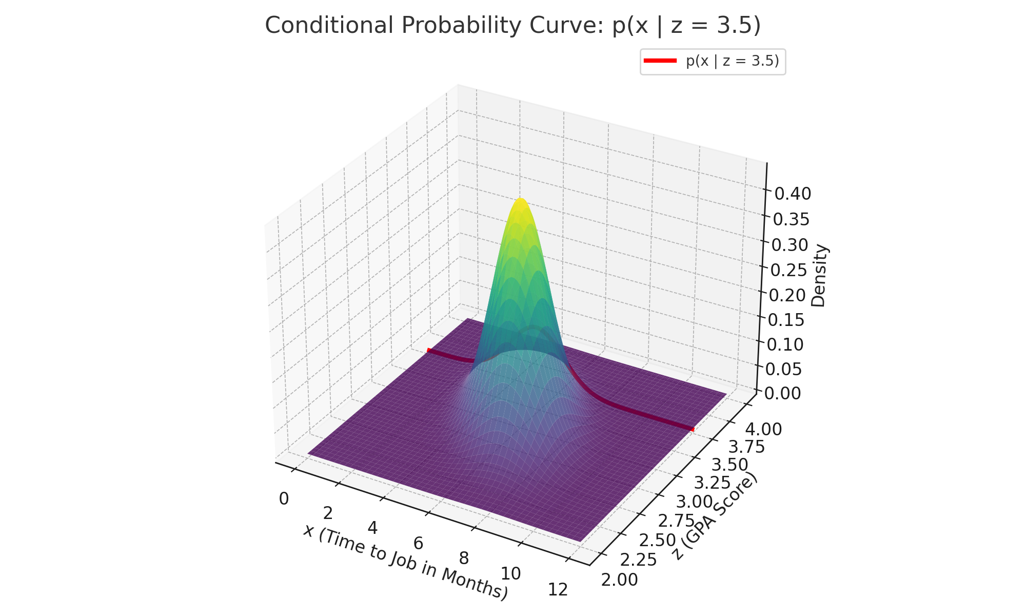
The whole plot surface represents the joint distribution $p(x, z)$, showing how GPA and job timing relate.

The red curve is a slice of that surface at $z = 3.5$ —
it shows the conditional distribution $p(x \mid z = 3.5)$.

So when we ask:

Among students with GPA = 3.5, how likely is it to get a job in 4 months?

You'd look up the height of that red curve at $x = 4$.
(Need I remind you that we’ll be using a range of x values to find the final probability here?)

Meaning of the Probability Density

The height of the curve at some point $x$, given say $z = 3.5$, has some value. Let's say:

This means that around 4 months, the likelihood of students getting jobs is high — 0.3 per month.

So if you want to know:

What's the probability that someone gets a job between 3.8 and 4.2 months?

That's a window of 0.4 months wide. Then:

So about 12% of students with GPA 3.5 get a job in that 0.4-month window.

The shape of the distribution surface in the above image is simply a visual representation of the frequencies of particular events occurring.

If the curve is at a higher height, then the variables corresponding to those height values have high occurrences.

This distribution helps understand, at a glance, how the different variable values are distributed. That’s it!

Of course, this example is also for the case of 2 variables only.
But if we are heading toward deep learning, then the number of variables can be very high.

That’s why it’s hard to visualize the high-dimensional operations happening there.

Level 3 — Sampling: Bringing Distributions to Life

So far, we've talked about distributions as shapes — as smooth landscapes where some regions are taller (more likely) and others shorter (less likely).

There are many different kinds of distributions that any data can follow.
The most important assumption we make is that we know the distribution to some extent.

In the deep learning world, we usually reach this state by learning the distribution — often at the expense of huge compute. This process is called model training (more on that later).

Even though the actual distribution can’t be learned 100% precisely, given a diverse and massive dataset, we assume that our model approximates this data distribution well enough.

But Now Comes a Very Powerful Question:

How do we actually use these distributions to create new examples of data?

This is where the concept of sampling enters.

What Does “Sampling” Even Mean?

Let's go back to our earlier red curve — the one that says:

Given a GPA of 3.75, here’s how job timings are spread out.

You can think of this curve as a rulebook that nature might use to decide who gets a job when.

Now suppose you want to simulate a new student:

What month will they get a job if their GPA is 3.5?

You don’t want to just guess randomly.
You want to follow the curve — make common things more likely, and rare things less likely.

That’s sampling.

Sampling Is Like Gravity: You Fall Where It’s Deepest

Imagine dropping marbles onto the curve. Where are they likely to land?

• Near the tall regions (say, around 4 months), they’ll pile up
• In flat zones (like 8 months), they’ll barely appear

If you drop 10,000 marbles and plot where they land,
the cloud of dots will recreate the shape of the original curve.

In simple terms:

The data reveals the distribution when plotted.
And the distribution creates data by sampling.

Sampling Is What Makes Generative Models “Generative”

This is the core of every generative model — whether it’s GPT, StyleGAN, or a diffusion model:

1. Learn a distribution from real data
2. Sample from that learned distribution
3. Output something new — a sentence, a face, a sound, etc.

It’s like saying:

“I’ve understood how the real world spreads things out.
Now let me use that understanding to imagine something similar — but fresh.”

Connecting Back to Bayes

Let’s not lose sight of our root formula:

From this, we learned to slice a joint distribution and get a conditional one.

Now, by sampling from that conditional distribution,
we can simulate possible x values, given some z.

And this act of:

“simulating x given z”
That’s literally the job of a generative model.

Whether:

• z is a label ("cat") and x is an image
• Or z is a prompt ("Once upon a time") and x is the next words

We're still doing:

You Already Understand Half of Generative AI

If you’ve followed along so far:

• You now understand how data is stored in a distribution
• How conditioned distributions carve out specific realities
• And how sampling gives us new data points

This is what generative models do — just at a much larger scale and in higher dimensions.

Level 4 — From Understanding to Imagination

We've talked a lot about how to interpret conditional probabilities, how to visualize distributions, and how to sample from them.
Now let's turn the corner.
Until now, we've mostly been asking questions like:

Given a GPA (z), how long does it take someone to get a job (x)?

But what if we flip it?
What if we want to generate new job timelines for imaginary students with realistic GPAs?
Or more generally:

Can we build a system that creates synthetic, but realistic data samples?

Welcome to the world of generative models — and yes, it all starts from Bayes' formula.

Quick Recap: Bayes' Rule

Let's again look at the first image in this blog (Bayes’ formula).
In plain English:

• p(z | x) = how likely the cause (z) is, given we saw some effect (x)
• p(x | z) = how likely the effect is, assuming a certain cause
• p(z) = how common that cause is overall
• p(x) = a normalizing term (makes sure probabilities add up to 1)

Now here's the twist:
Even though Bayes' rule helps us compute p(z | x) — meaning, given an observation, guess its hidden cause —
we can also reverse the flow and generate data by first imagining a cause, then simulating the effect.
And that, right there, gives us a generative model.

A Simple Generative Model: Step-by-Step

Let’s stick to our example:

• z = GPA of a student
• x = how many months it takes to get a job

We already visualized p(x | z) — the red curve sliced out from the 3D joint surface.
We also assumed we know how GPAs are distributed in the population — say, a bell curve centered at 3.3.
Let’s use that to generate synthetic student data.

Step 1: Sample a GPA

We start by picking a random GPA value from p(z) — maybe it lands at 3.75.
Think of it like: we imagined a student who randomly popped out of the real-world GPA distribution.

Step 2: Given that GPA, Sample Job Timing

Now that we’ve fixed z = 3.75,
we go to the red curve p(x | z = 3.75) and sample a job-finding time from it — maybe it lands at 4.2 months.

That’s one synthetic data point:

(GPA = 3.75, job = 4.2 mo)

Repeat this 100 times, and you get a full fake dataset that feels just like real students.

That’s a Generative Model!

Let’s write down what we just did in math:

A Familiar Example

Your phone suggesting the next word while you're typing a message.
You write:

"I hope you're having a…"

Suddenly, your keyboard suggests:

great, nice, wonderful

What just happened?

Your phone used a language model — a type of generative model — to guess what word x is most likely to follow the previous words z.

Mathematically, it used:

The probability of next word x, given the context z.

Behind the Scenes: A Two-Step Sampling

1. It fixes the context (the sentence so far) → that’s our z
2. It then samples from a distribution over the next word → that’s p(x | z)

You don’t see this math.
You just see suggestions that feel right.

But under the hood?
It’s Bayes all the way down.

Model Training

In our example, we assumed we knew both:

• p(z) — the natural spread of GPAs in the population
• p(x | z) — the likelihood curve of job timings for each GPA

But in real life?
We don’t know these distributions.
We only have data.
So, what do we do?
We learn them.
We approximate them using powerful neural networks.
That leads us into methods like:

Variational Autoencoders (VAEs)
→ where we learn p(x | z) as a decoder, and approximate p(z | x) to help train it

Diffusion Models
→ which gradually destroy and then reconstruct samples, reversing from noise (cause) to data (effect)

GANs (Generative Adversarial Networks)
→ which try to sample from p(x) directly by tricking a critic

But even these complex models are just variations of the same theme:

Start from a latent cause (z)
Generate an observable effect (x)

And that's exactly what Bayes’ rule encourages us to think about.

TL;DR

• What p(x | z) really means
• How it's built from joint probability p(x, z)
• That every distribution has a shape
• That sampling from a distribution = generating new data
• That generative models just sample x ~ p(x | z)
• That Bayes' rule is the quiet engine behind it all

References

Introspective knowledge gained so far.

Also Published on Medium

Prefer reading on Medium?

👉 Read this article on Medium